Reservoir Sampling and Randomized Algorithms

How the randomized algorithms work and its implementation in streaming systems

Randomized Algorithm

Randomized algorithm applies a certain level of randomness as part of the logic. It usually uses uniform random(Each element from a N dataset has 1/N probability being chosen) to define the behaviour of auxiliary input in the hope of achieving good performance in average case;

The randomized algorithms are random in following aspect:

1. The operation of actual problem is random;
2. The computing complexity of the problem is a random variable;
3. The algorithm output is random;(might be right/wrong);

a. choose one element randomly

For the ith element, we must have (1/i) probability of choosing and (1-1/i) not choosing;

// One element
// Proof of uniform random
// for ith item, the probability of being chosen
1/i * (1 - 1/(i+1)) * (1 - 1/(i+2)) * ... * (1 - 1/n)
= 1/i * i/(i+1) * (i+1)/(i+2) * ... * (n-1) / n
= 1/n 

b. choose k elements randomly

For the ith element, the probability of being chosen k/i, the probability of not being chosen (1-k/i);

// K elements
// Proof of uniform random
// for ith item, the probability of being chosen
k/i * (1 - k/(i+1) * 1/k) * (1 - k/(i+2) * 1/k) * ... * (1 - k/n * 1/k)
= k/i * (1 - 1/(i+1)) * (1 - 1/(i+2)) * ... * (1 - 1/n)
= k/i * i/(i+1) * (i+1)/(i+2) * ... * (n-1) / n
= k/n 

1. Reservoir sampling

Reservoir sampling is a family of randomized algorithms for choose a simple [random sample] [without replacement of k items] from a population of [unknown size n] in a [single pass] over the items.

NOTE:

• size n here usually cannot fit into main memory;
• n is unknown, revealed over the time; otherwise it would be too easy;
• time complexity required is O(N);
• probability of each item being chosen must be k/n;

Simple Algorithm

The commonly used algotihm that is simple but slow, known as: Algorithm R;

/**
 * Algorithm R works by maintaining a reservoir size of k, 
 * 1. which initially contains the first k items of the input;
 * then iterates over the remaining items until the input is exhausted.
 * 2. when reaches the ith item
 *   a. if i >= k, random choose d in [0, i]
 *      if d is within [0, k -1], use ith item to replace dth item in reservoir; 
 * 3. repeat second step;
 */

int[] reservoir = new int[k];

for (int i = 0; i < reservoir.length; i++)
{
    reservoir[i] = dataStream[i];
}

for (int i = k; i < dataStream.length; i++)
{
    // random integer in [0, i];
    int d = rand.nextInt(i + 1);
    // if integer is within [0, m-1]，then replace reservoir
    if (d < k)
    {
        reservoir[d] = dataStream[i];
    }
}

CONS: asymptotic running time is thus O(n), which causes the algorithm to be unnecessarily slow if the input population is large.

Distributed/Parallel Reservoir Sampling

In idistributed systems, main memory & IO ops would be the bottleneck; So for the data of a super large scale, we could improve the overall performance using parallel algorithm:

1. Assume we have m machines, divide the stream into m data stream, every single machine process one stream of m samples, then note down as N1, N2, ..., Nk, ... NK(assume m < Nk>) => N1 + N2 + N3 + … + NK = N;
2. Choose a random number d from [1, N]: a. if d < N1, then replace (1/m) from the first machine, …; repeat m times;

=> m / N

Implementation

Because the reservoir sampling has O(N) time complexity and O(M) space complexity, it is usually adopted in streaming systems where statistical sampling is required. For example, random output n lines from a large-scale dataset;

For algorithm lovers, you could also find some common problems like： linked list random node, pick random index;

Limitations

Reservoir sampling makes the assumption that the desired sample fits into main memory, often implying that k is a constant independent of n.

ref: wiki: reservoir sampling#limitations

In applications where we would like to select a large subset of the input list (say a third, i.e. k=n/3), other methods need to be adopted. Distributed implementations for this problem have been proposed.

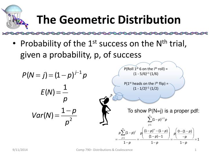
2. Geometric Distribution

Time Complexity O(K + Klog(N/K))

3. Fisher–Yates shuffle

The Fisher–Yates shuffle is used to generate a random permutation of a finite sequence, meaning to shuffle the sequence;

So choose K items randomly from the sequence just equals to shuffling the deck of size k;

-- To shuffle an array a of n elements (indices 0..n-1):
for i from n−1 downto 1 do
     j ← random integer such that 0 ≤ j ≤ i
     exchange a[j] and a[i]

Reference

• Reservoir sampling;
• randomized algorithms;
• random functions
• Fisher–Yates shuffle
• Geometric Distribution